Top 3 Most Common Inventory Control Policies

By Xabier Lizartzategi, Jan , 2021
This blog defines and compares the three most commonly used inventory control policies. It should be helpful both to those new to the field and also to experienced people contemplating a possible change in their company’s policy. The blog also considers how demand forecasting supports inventory management, choice of which policy to use, and calculation of the inputs that drive these policies. Think of it as an abbreviated piece of Inventory 101.
Scenario
 You are managing a particular item. The item is important enough to your customers that you want to carry enough inventory to avoid stocking out. However, the item is also expensive enough that you also want to minimize the amount of cash tied up in inventory. The process of ordering replenishment stock is sufficiently expensive and cumbersome that you also want to minimize the number of purchase orders you must generate. Demand for the item is unpredictable. So is the replenishment lead time between when you detect the need for more and when it arrives on the shelf ready for use or shipment. Your question is “How do I manage this item? How do I decide when to order more and how much to order?” When making this decision there are different approaches you can use. This blog outlines the most commonly used inventory planning policies: Periodic Order Up To (T, S), Reorder Point/Order Quantity (R, Q), and Min/Max (s, S). These approaches are often embedded in ERP systems and enable companies to generate automatic suggestions of what and when to order. To make the right decision, you’ll need to know how each of these approaches are designed to work and the advantages and limitations of each approach.
Periodic review, order-up-to policy
The shorthand notation for this policy is (T, S), where T is the fixed time between orders and S is the order-up-to-level.
When to order: Orders are placed like clockwork every T days. The used of a fixed reorder interval is helpful to firms that cannot keep track of their inventory level in real time or who prefer to issue orders to suppliers at scheduled intervals.
How much to order: The inventory level is measured and the gap computed between that level and the order-up-to level S. If the inventory level is 7 units and S = 10, then 3 units are ordered.
Comment: This is the simplest policy to implement but also the least agile in responding to fluctuations in demand and/or lead time. Also, note that, while the order size would be adequate to return the inventory level to S if replenishment were immediate, in practice there will be some replenishment delay during which time the inventory continues to drop, so the inventory level will rarely reach all the way up S.
 Continuous review, fixed order quantity policy (Reorder Point, Order Quantity)
The shorthand notation for this policy is (R, Q), where R is the reorder point and Q is the fixed order quantity.
When to order: Orders are placed as soon as the inventory drops to or below the reorder point, R. In theory, the inventory level is checked constantly, but in practice it is usually checked periodically at the beginning or end of each workday.
How much to order: The order size is always fixed at Q units.
Comment: (R, Q) is more responsive than (S, T) because it reacts more quickly to signs of imminent stockout. The value of the fixed order quantity Q may not be entirely up to you. Often suppliers can dictate terms that restrict your choice of Q to values compatible with minima and multiples. For example, a supplier may insist on an order minimum of 20 units and always be a multiple of 5. Thus orders sizes must be either 20, 25, 30, 35, etc. (This comment also applied to the two other inventory policies.)
Continuous review, order-up-to policy (Min/Max)
The shorthand notation for this policy is (s, S), sometimes called “little S, big S) where the reorder point and S is the order-up-to level. This policy is more commonly called (Min, Max).
When to order: Orders are placed as soon as the inventory drops to or below the Min. As with (R, Q), the inventory level is supposedly monitored constantly, but in practice it is usually checked at the end of each workday.
How much to order: The order size varies. It equals the gap between the Max and the current inventory at the moment that the Min is reached or breached.
Comment: (Min, Max) is even more responsive than (R, Q) because it adjusts the order size to take account of how much the inventory has fallen below the Min. When demand is either zero or one units, a common variation sets Min = Max -1; this is called the “base stock policy.”
Another policy choice: What happens if I stock out?
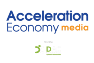
As you can imagine, each policy is likely to lead to a different temporal sequence of inventory levels (see Figure 1 below). There is another factor that influences how events play out over time: the policy you select for dealing with stockouts. Broadly speaking, there are two main approaches.
Backorder policy: If you stock out, you keep track of the order and fill it later. Under this policy, it is sensible to speak of negative inventory. The negative inventory represents the number of backorders that need to be filled. Presumably, any customer forced to wait gets first dibs when replenishment arrives. You are likely to have a backorder policy on items that are unique to your business that your customer cannot purchase elsewhere.
Loss policy: If you stock out, the customer turns to another source to fill their order. When replenishment arrives, some new customer will get those new units. Inventory can never go below zero. Choose this policy for commodity items that can easily be purchased from a competitor. If you don’t have it in stock, your customer will most certainly go elsewhere.
The role of demand forecasting in inventory control
Choice of control parameters, such as the values of Min and Max, requires inputs from some sort of demand forecasting process.
Traditionally, this has meant determining the probability distribution of the number of units that will be demanded over a fixed time interval, either the lead time in (R, Q) and (Min, Max) systems or T + lead time in (T, S) systems. This distribution has been assumed to be Normal (the famous “bell-shaped curve”). Traditional methods have been expanded where the demand distribution isn’t assumed to be normal but some other distribution (i.e. Poisson, negative binomial, etc.)
These traditional methodologies have several deficiencies.
- First, it usually ignores the problem of undershoot, in which demand drops inventory not just to the reorder point but below it. Assuming no undershoot leads to overestimates of service levels and fill rates.
- Second, the probability distribution of demand is very often not even close to “bell-shaped” or whatever assumed distribution was selected – especially for items with intermittent demand such as spares and service parts.
- Third, accurate estimates of inventory operating costs require analysis of the entire replenishment cycle (from one replenishment to the next), not merely the part of the cycle that begins with inventory hitting the reorder point.
- Finally, replenishment lead times are typically unpredictable or random, not fixed. Many models assume a fixed lead time based on an average, vendor quoted lead time, or average lead time + safety time.
Fortunately, better inventory planning and inventory optimization software exists based on generating a full range of random demand scenarios, together with random lead times. These scenarios “stress test” any proposed pair of inventory control parameters and assess their expected performance. Users can not only choose between policies (i.e. Min, Max vs. R, Q) but also determine which variation of the proposed policy is best (i.e. Min, Max of 10,20 vs. 15, 25, etc.) Examples of these scenarios are given below.
The process of ordering replenishment stock is sufficiently expensive and cumbersome that you also want to minimize the number of purchase orders you must generate
Choosing among inventory control policies
Which policy is right for you? There is a clear pecking order in terms of item availability, with (Min, Max) first, (R, Q) second, and (T, S) last. This order derives from the responsiveness of the policy to fluctuations in the randomness of demand and replenishment. The order reverses when considering ease of implementation.
Inventory cost can be expressed either as inventory investment or inventory operating cost. The former is the dollar value of the items waiting around to be used. The latter is the sum of three components: holding cost (the cost of the “care and feeding of stuff on the shelf”), ordering cost (basically the cost of cutting a purchase order and receiving that order), and shortage cost (the penalty you pay when you either lose a sale or force a customer to wait for what they want).
Service is usually measured by service level and fill rate. Service level is the probability that an item requested is shipped immediately from stock. Fill rate is the proportion of units demanded that are shipped immediately from stock. As a former professor, I think of service level as an all-or-nothing grade: If a customer needs 10 units and you can provide only 9, that’s an F. Fill rate is a partial credit grade: 9 out of 10 is 90%.
When you decide on the values of inventory control policies, you are striking a balance between cost and service. You can provide perfect service by keeping an infinite inventory. You can hold costs to zero by keeping no inventory. You must find a sensible place to operate between these two ridiculous extremes. Generating and analyzing demand scenarios can quantify the consequences of your choices.
A demonstration of the differences between two inventory control policies
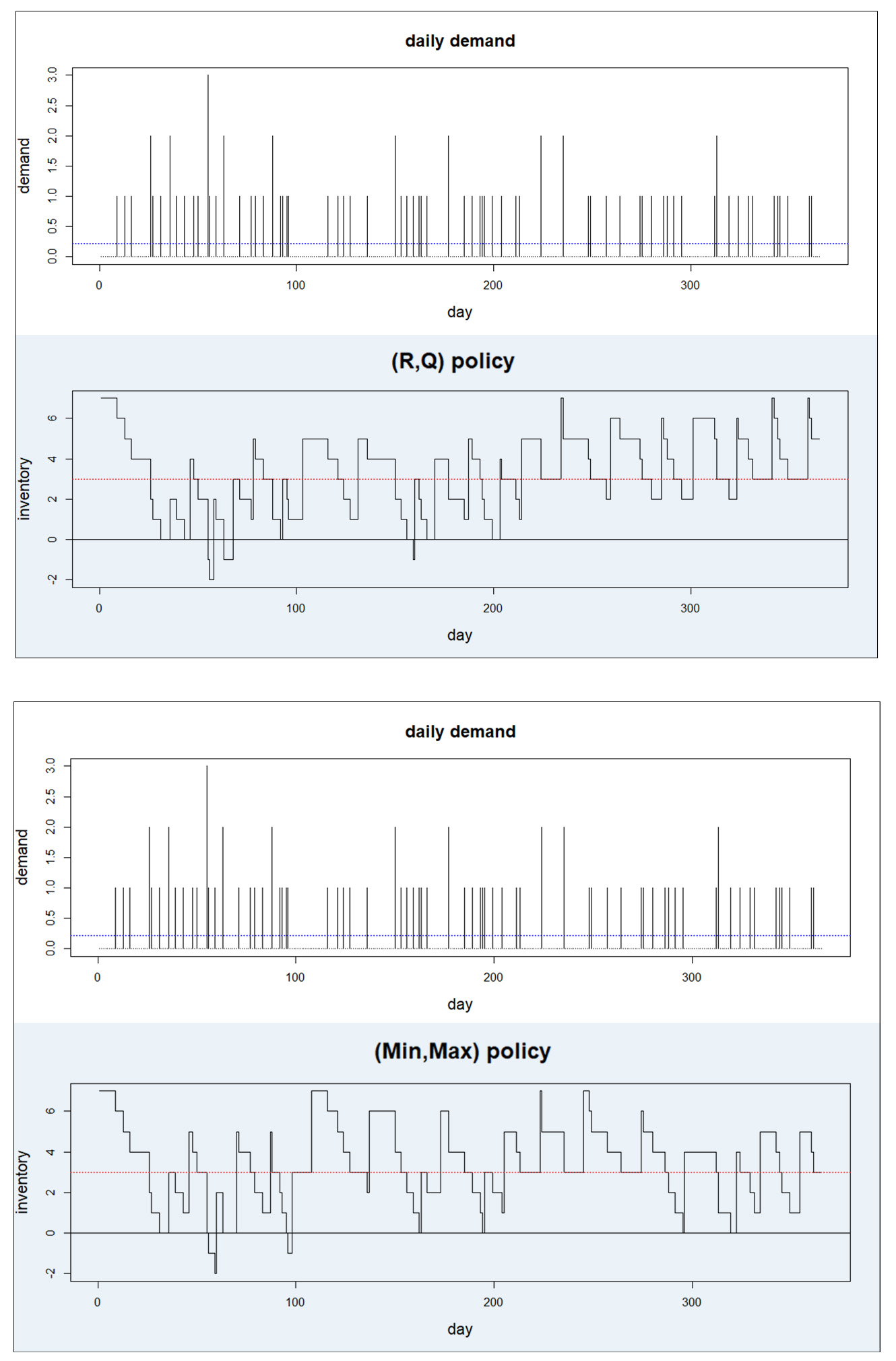
Figure 1: Comparison of daily on-hand inventory under two inventory policies
Role of Inventory Planning Software
Best of Breed Inventory Planning, Forecasting, and Optimization systems can help you determine which type of policy (is it better to use Min/Max over R,Q) and what sets of inputs are optimal (i.e. what should I enter for Min and Max). Best of breed inventory planning and demand forecasting systems can help you develop these optimized inputs so that you can regularly populate and update your ERP systems with accurate replenishment drivers.
Summary
We defined and described the three most commonly used inventory control policies: (T, S), (R, Q) and (Min, Max), along with the two most common responses to stockouts: backorders or lost orders. We noted that these policies require successively greater effort to implement but also have successively better average performance. We highlighted the role of demand forecasts in assessing inventory control policies. Finally, we illustrated how choice of policy influences the day-to-day level of on-hand inventory.