Categories: Power Platform UG, User Group Communities
Power BI should definitely be in your business intelligence toolkit, and when you add in R or Python, you can unlock "superpower features". These features expand the possibilities for machine learning, forecasting, and advanced analytics.
To showcase the power of these advanced capabilities, I will walk you through the use of the Python PyCaret Time Series module in Power BI and create a forecast analysis for the price of a commodity.
Now, if you are like me, just visualizing a forecast is not enough to answer business questions. So, I was wondering how to ask business questions by adding time intelligence to the forecast. What I found was this can be done by combining a bit of DAX with the forecast performed by the PyCaret package and its Time Series module.
If you would like to learn more Machine Learning techniques, then I would recommend my book Machine Learning en Power BI with R and Python, which you can get in English and Spanish - and soon in Portuguese. 10% of our revenues will be donated to the PyCaret team.
For the sake of this example, I will not go into making a very accurate model. I will focus more on the solution and will leave the reader the task of researching how to make a more accurate model; something that is not complex with the PyCaret Time Series Model.
Now, on to the good stuff!
Before starting, install PyCaret and specifically the Time Series module. To do so, I advise you to read these instructions on how to install PyCaret Time Series Module. PyCaret works very well with Python 3.8.
The dataset to use is within a CSV file called ‘commodity_price.csv’ (you can download the sample file here), which is a time series with the price of a given commodity from January 6, 2017, to date, with daily data points. This dataset contains only two columns, “date” and “price”, and it looks like this:
It is highly recommended that you create a new virtual environment to install the PyCaret Time Series Module, as it currently has some version conflicts with PyCaret original package. The PyCaret team is working hard to integrate everything under one single package, but nowadays, it has to be in separate environments.
You can read about how to create a new Anaconda virtual environment here .
Once a new virtual environment is created and the PyCaret Time Series Module is installed, it is necessary to sync up Power BI with the new virtual environment, so all functionalities can be used within Power BI.
In my example, I created an Anaconda virtual environment called “pycaret_ts”. To sync up this new virtual environment with Power BI
Now that Power BI is ready, so are we! Let’s do some forecasting.
As we select “Transform data” in Power BI desktop, we open the Power Query environment, where we will perform the forecasting. Before working with time series, it is very important that the data is sorted in descending order. Once there, and after loading the original dataset, let’s create a copy of it to be renamed “forecast.”
Let’s make a forecast for the next 60 days after the last data point that is available in the dataset. So, after selecting the “forecast” query, select Transform > Run Python Script and insert the following code:
import pandas as pd
import numpy as np
from pycaret.time_series import *
df = dataset[['price']]
setup(df, fh = 60, fold = 4, session_id = 100, seasonal_period = 'D', html = False, verbose = False)
model = create_model('auto_arima', verbose = False)
fcst = predict_model(model, alpha = 0.1, return_pred_int = True)
fcst = pd.DataFrame(fcst)
fcst['day_added'] = np.arange(len(fcst))
fcst['type'] = pd.Series('forecast', index=df.index, dtype='category')
fcst
Once inserted looks the code appears as such:
Once executed, Power Query returns all the tables and data frames generated by the code. In this case, the one that contains the forecast is called ‘fcst’; so, let’s expand it. At the forecast table, let’s rename the column “y_pred” to “price”. The forecast table looks like this:
There are a few things that need to be done before selecting “Close & Apply”. Go back to the original dataset named “commodity_price” and add a new custom column named “type” with the only value of “historical.” To do this, just go to Add Column > Custom Column and create a new column with those features.
Now, those tables are ready to be appended. So, let’s go to Home > Append Queries > Append Queries as new, and select “commodity_price” as the First table and “forecast” as the Second table, like this:
A new table called ‘Append1’ is now created. So, let’s rename it to “consolidated”, as this new table contains both historical data, commodity_price, forecast data, and the forecast.
There is more transformation that needs to be done within the “consolidated” table”
After all those transformations, this is how the “consolidated” table looks like:
Now, everything is ready to go, so let’s hit “Close & Apply” and let everything be uploaded to memory. Here is the visual result:
Now comes the nice part. As this forecast data is part of the data model, it is possible to create DAX measures to calculate the expected growth of the price with the forecast, or even the Standard Moving Average of the price, but now including the forecast.
Let’s calculate the Standard Moving Average of 60 days, but adding a new measure using the following DAX measure:
SMA 60d = CALCULATE( AVERAGEX( Append1, Append1[price] ),
DATESINPERIOD( Append1[fecha], LASTDATE( Append1[fecha] ), -60, DAY ) )
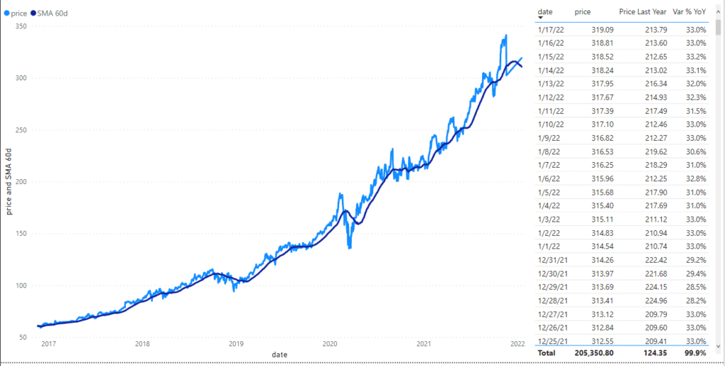
Something else that is an interesting capability is the option to calculate the growth rate of the price day by day. For example, choosing to compare the same day of last year to the current growth rate.
To do so, it is necessary to create several DAX measures:
Price Last Year = CALCULATE( AVERAGE( Append1[price] ), SAMEPERIODLASTYEAR( Append1[fecha] ) )
Var % YoY = DIVIDE( ( SUM( Append1[price] ) - Append1[Price Last Year] ), SUM( Append1[price] ) )
Let’s look at the result:
Now we can estimate the growth of forecasted points against the same price value one year ago.
This is the great advantage of having forecast points in the same data model as it is possible to add intelligence to the forecast.
There was a problem reporting this post.
Please confirm you want to block this member.
You will no longer be able to:
Please note: This action will also remove this member from your connections and send a report to the site admin. Please allow a few minutes for this process to complete.
Here you will find a wealth of information created for people that are on a mission to redefine business models with cloud techinologies, AI, automation, low code / no code applications, data, security & more to compete in the Acceleration Economy!